Liquid/liquid equilibria

Phase equilibria play a central role for the production, characterization and application of polymers. In the present context this is above all true for the determination of molar masses M and of parameters quantifying the interaction with other components, like solvents or polymers of different chemical or architectural structure. In case of the classical determination of M by means of osmometry it is the equilibrium between the solution and the pure solvent; with GPC the phases are a stationary and a mobile one.

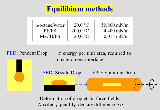
Closely related to the liquid/liquid phase equilibria is the interfacial tension \(\sigma\), which represents the energy required to create 1 \({{\rm{m}}^2}\) of new interface. This property is also defined as the partial derivative of the Gibbs energy with respect to the area of the interface between the coexisting liquids, keeping all other variables constant. The present chapter starts with brief reports on measurement techniques and theoretical tools. This part is then followed by the discussion of various topics, which were and are of special interest to us.

Experimental methods: The most reliable manner to obtain information on liquid/liquid phase equilibria rests on a detailed analysis of the coexisting phases. This method is, however, quite elaborate and quicker ways are often preferred. Turbidity measurements are most widely used, where the transition from a fully transparent solution to a turbid one is often monitored by the naked eye. An apparatus for automated turbidity titration turned out to be particularly helpful, among other things for the analysis of copolymers[^221]. It is obvious that all optical methods fail if the coexisting phases are iso-refractive. In such cases phase separation can also be precisely monitored by DSC calorimetry[^069]. The viscometric monitoring[^037] [^048] of the segregation of a further phase represents another versatile method for the study of liquid/liquid demixing. More details are provided in the section "Interrelation of thermodynamic and of flow effects".

Interfacial tensions \(\sigma\) can be determined by studying the deformation of tiny droplets in gravitational fields. "Spinning drop" and "sessile drop" are the most common methods. We have applied these techniques to polymer solutions[^125] [^154], as well as to polymer blends[^141] [^177] [^185] [^139].

Theoretical modeling: Many fundamental experimental observations with liquid/liquid phase equilibria can already be rationalized by means of the original Flory-Huggins theory. However, a quantitative description requires considerably more sophisticated approaches. The literature proposes several, where most of them treat special problems adequately, but lack generality. A procedure that does not require analytical expressions for the composition dependence of the Gibbs energy of mixing turned out to be helpful[^159a]. The method is briefly depicted in the following chart, showing the reduced Gibbs energy of mixing for a binary system that separates into two liquid phases within a characteristic composition range.

The red curve stands for the Gibbs energies of the (in some ranges hypothetical) homogenous mixtures; by means of very short "test tie-lines" it is checked, whether a further reduction of the Gibbs energy can be achieved by a supposed demixing or whether homogenization takes place spontaneously. In this manner it is possible to distinguish between unstable, meta-stable and stable regimes.

Amongst the theoretical approaches yielding analytical expressions for the composition dependence of the Gibbs energies of mixing, the following Ansatz turned out to be particularly helpful. It subdivides the process of solvent addition to polymer solutions into two clearly distinguishable steps: the insertion of solvent between two polymer segments and the subsequent rearrangement of the components to assume their equilibrium positions. The details of this approach are presented in the section "Interaction parameters". It reproduces binodal and spinodal lines very accurately[^248] at low temperatures (UCSTs) and at high temperatures (LCSTs). It also enables the prediction of (endothermal) theta temperature as a function of pressure. Furthermore it can tentatively explain the reasons for anomalous demixing [^263], i.e. the existence of two critical conditions for liquid/liquid equilibria within one and the same system.

Interfacial tension \(\sigma\): We have studied the correlation of \(\sigma\) with the details of the composition dependence of the Gibbs energy of mixing[^228] and introduced the concept of a "hump energy"[^152] [^161] as illustrated in the next chart.

Experimental results: The best studied question is the influences of chain length on the sensitivity towards liquid/liquid phase separation. Inevitably and above all in the context of polymer fractionation, we have also dealt with these effects[^029] [^033] [^035] [^044] [^215] [^244] [^256]. For a number of reasons it is often helpful to dissolve polymers in more than one low molecular weight liquid. If this mixture consists of a good and of a poor solvent, it is for instance possible to vary the solvent power gradually and continuously. This feature is of central importance for a continuous large-scale fractionation of polymers with respect to polymer mass or/and chemical composition as described in the section “Continuous Polymer Fractionation”. It is also the basis for the preparation of membranes by means of the phase inversion process, e.g. directly from solutions of unsubstituted cellulose[^257]. More information on non-additivity effects of the present nature and their interpretation is given in references [^023] [^025] [^039] and [^239].

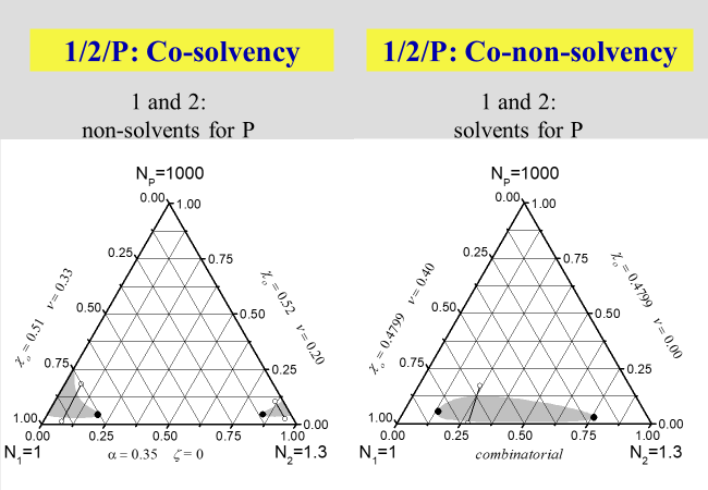
Another interesting phenomenon, which is well known since the early days of polymer science, is "cosolvency" i.e. the fact that certain combinations of non-solvents may create good solvents. The opposite behavior, namely the formation of a precipitant by combining two favorable solvents, the so-called " co-nonsolvency ", on the other hand, was detected much later[^039]. A special case exists if the formation of homogeneous polymer solutions in mixed precipitants is bound to the application of pressure. This phenomenon, called "true cosolvency", will be discussed in the next section dealing with pressure.

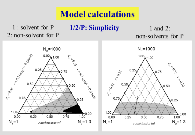
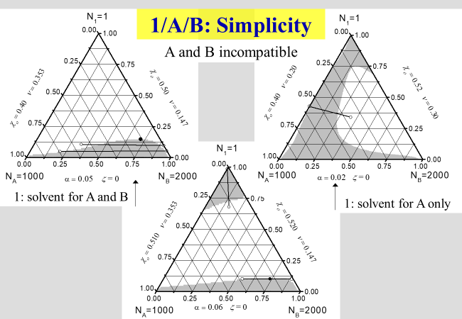
One of the strengths of the approach subdividing the dilution process into two clearly separable steps mentioned above, consists in the ability to rationalize all principal phenomena observed with ternary systems[^239]. In the next charts, showing the results of such calculations, numbers stand for low molecular weight components and letters for polymers; N specifies the number of segments of the different components, \(\alpha\) quantifies the part of the interaction parameter \(\chi\), which stems from the separation of two polymer segments at infinite dilution by inserting a solvent molecule between them. The parameter \(\zeta\), on the other hand, describes the effects caused by the rearrangement of the components after dilution. The parameter \(\nu\) is required to quantify the effects caused by the geometrical dissimilarity of solvent molecules and polymer segments, and \({\chi _{\rm{o}}}\) stands for the Flory-Huggins interaction parameter in the limit of infinite dilutions.

The next two charts show the results of the application of the present approach to solutions of polymers in mixed solvents, where the first one describes the demixing behavior in the absence of special interactions that may lead to non-additivity effects. The second chart then deals with the phenomena of cosolvency (two non-solvents may act as solvent, if mixed properly) and of co-nonsolvency (mixing two good solvents may - at certain ratios - create a non-solvent).

How the phase diagrams may look like in the case a polymer blend is dissolved in a single solvent is displayed in the next two charts. The first chart describes the simplest possible behavior again .

The following chart models an experimentally observed phase diagram[^297], namely the formation of islands of immiscibility upon the addition of solvent to a pair of compatible polymers.

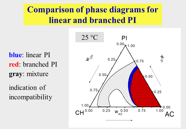
Poorly defined polymers: One problem out of this area concerns the demixing of samples with broader molecular weight distribution. The effects with respect to phase separation are discussed in the context of "Continuous polymer fractionation". Another type of unexpected behavior can result from admixtures of high molecular components that differ in their chemical or/and molecular architecture from the polymer of interest. An example for such effects[^284] is presented below. Despite very similar miscibility gaps of linear and of branched polyisoprene in the mixed solvent cyclohexane + acetone, their mixtures exhibit much larger two-phase areas.

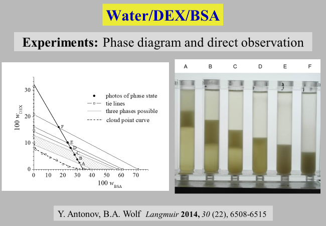
Biopolymer containing systems: Their phase separation behavior is in many cases much more complicated than that of linear homopolymers as demonstrated[^321] for the ternary system water/dextran/BSA (bovine serum albumin). Depending on the ratio of the two polymers, the system phase separates into two or three liquid phases, respectively.

Pressure influences: This often-neglected variable was and still is of particular interest to us. It becomes above all important for very volatile, i.e. compressive liquids and gaseous components. One of the most remarkable effect concerns the fact that pressure may generate polymer incompatibility in some cases[^244] but lead to compatibility in others[^232]. An example for the complex influences is given in the next chart showing the phase separation behavior of the system diethyl ether/acetone/polystyrene[^029][^030]. The mixtures are two-phase outside the closed curves.

Among the systems that behave as expected, we have for instance studied solutions of narrowly distributed polyethylene in n-hexane[^254] and of polybutadiene in n-butane[^264].