Influences of T, p and shear

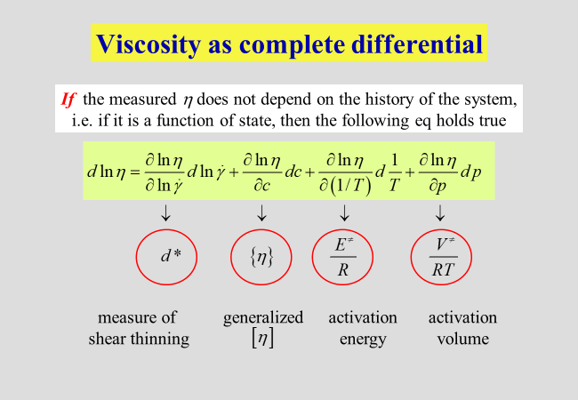
As long as the viscosity represents a function of state, the following relations hold true. Concentration influences have already been dealt with in the preceding chapter. Here we are starting with typical examples for the dependencies on pressure and on temperature.

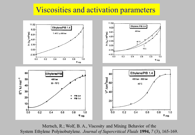
Pressure and temperature influences: Some solvents require higher pressures to form homogeneous mixtures with polymers; the systems ethylene/polyethylene[^193], carbon dioxide/poly dimethyl siloxane[^150] or ethylene/polyisobutylene[^148] are examples. For the last system the necessary pressures are on the order of 200 to 500 bar in the temperature range from 30 to 70 °C. It appears noteworthy in this context that – for low molecular weight compounds and as a rule of the thumb – the activation energies are approximately one third to one fourth of the heats of vaporization and the activation volumes one third to one fourth of the molar volumes. In view of the higher cohesive energy densities and of the large volume of the flow units in case of macromolecules, it is not surprising that the activation parameters are considerably bigger as shown in the following figures.

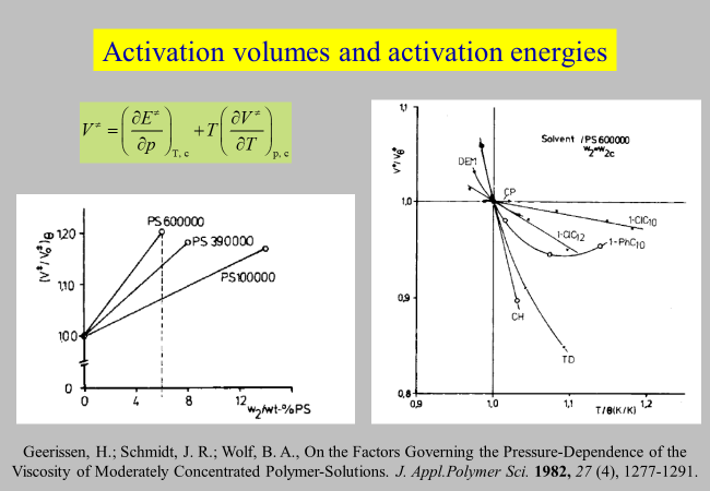
The next chart compares the influences of p and T on the viscosities of some typical systems, for solvents that are liquid under ambient conditions. Measurements were carried out for eight polystyrene samples in theta solvents at the respective critical compositions[^053]. The results show that the volumes of activation exceed that of the pure solvent by typically 10- % under these conditions. As indicated in the graph, activation volumes and activation energies are interdependent. The reliability of the experimental data can therefore always be controlled by checking whether they obey the displayed equation.

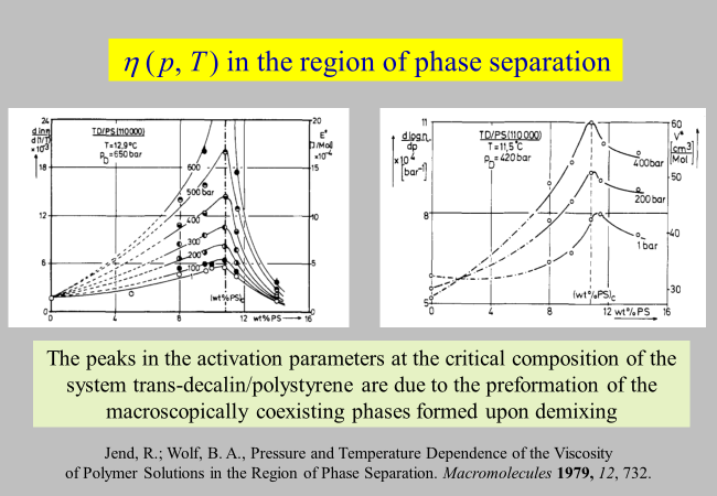
The p and T influences on the viscosities of polymer solutions we have discussed so far were unbiased by special effects. One important example for additional contributions[^041] concerns the formation of particular structures, eventually leading to phase separation as demonstrated below.

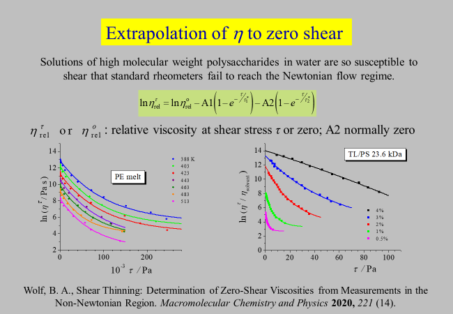
Extrapolation to zero shear: We are now turning to the effects of shear rate. There are two aspects that interests us most: The extrapolation of data obtained at finite \(\dot \gamma\) to zero shear and a better understanding of the omnipresent phenomenon of shear thinning. For some systems or conditions, it is impossible or impracticable to measure the zero shear viscosity directly. For that reason we have developed an extrapolation procedure as described in the following chart. The approach uses - in its simplest and normal case - the following adjustable parameters: The zero-shear viscosity of the system, a characteristic shear stress, quantifying its susceptibility towards shear thinning, and a dimensionless parameter stating the magnitude of the effect. As a by product this data treatment discloses two phenomena not reported so far: A qualitative change in the efficacy of shear stress at a characteristic concentration and the occurrence of two different disentanglement mechanisms in thermodynamically unfavorable solvents. The procedure is exemplified for polyethylene melts and for solutions of polystyrene in toluene.

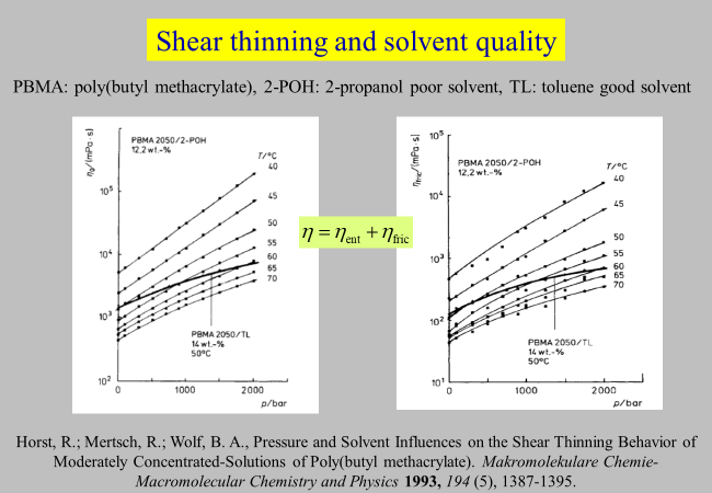
Shear thinning: For almost all polymer solutions the viscosity decreases with rising shear rate. This phenomenon is in many cases well described quantitatively by Graessley’s theory (W. W. Graessley, Adv. Polym. Sci. 16, 1 (1974)) but fails in others, particularly for solvents of marginal thermodynamic quality. We wanted to find an explanation for this observation by means of an approach that separates the viscosity \(\eta\) into an entanglement contribution \({\eta _{{\rm{ent} }}}\) and a frictional contribution \({\eta _{{\rm{fric}}}}\)[^057], [^058], [^132]. The following chart displays some pertinent results for the system 2-propanol/poly(butyl methacrylate)