Interaction parameters

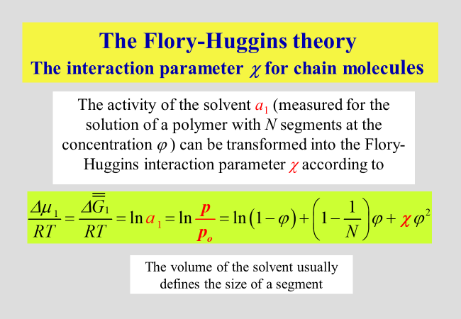
The classical thermodynamics of polymer-containing liquid mixtures was developed independently by P.J. Flory and M. L. Huggins. It is based on the well-known lattice model qualitatively formulated by K. H. Meyer, who pointed out the effect of the differences in molecular size of polymers and low molecular weight compounds with respect to the entropy of mixing. The quantitative calculation of the entropy of mixing led to the introduction of a dimensionless quantity, the so-called Flory-Huggins interaction parameter \(\chi\), for the thermodynamic description of polymer solutions. It was evident from the beginning that \(\chi\) is a function of T, however at first \(\chi\) was considered to be independent of polymer concentration. Subsequent experiments have shown the necessity to treat \(\chi\) as a function of composition. Furthermore, \(\chi\) also depends on \({M_2}\) (the molecular weight of the polymer), not only at high dilution, but even in the range of large polymer concentrations [^162].

The Flory-Huggins interaction parameter \(\chi\) - as used today - is for solutions of homopolymers in low molecular weight liquids defined in the following way, where \({p_1}\) and \({p_{1,{\rm{o}}}}\) are the vapor pressure of the solvent above the solution and that of pure solvent, respectively. In case the gas phase deviates from ideality, fugacities need to be used instead of vapor pressures.

Meanwhile individual values of Flory-Huggins interaction parameters have been tabulated for many customary polymer/solvent systems under special conditions[^187]. The current presentation is not concerned with such details, but confines itself to two approaches we have developed. Information on the behavior of specific systems can be obtained by searching the section "Publications".

For a quantitative description the Gibbs energy of mixing as a function of composition in terms of the Flory-Huggins interaction parameter we have used two fundamentally different lines of attack: A molecular modelling, dividing the dilution process into two separate steps, and a phenomenological approach attempting a unified description of the multitude of different macromolecular compounds.

Molecular approach[^305b]. The Flory-Huggins interaction parameter, \(\chi\), standing at the begin of the theoretical thermodynamic description of polymer containing systems, has been refined in several steps.

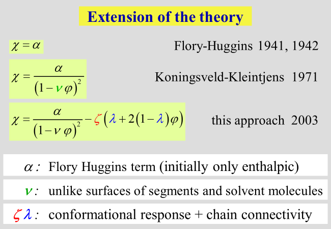
\(\chi\) was meant to account for all effect of separating two polymer segments by the insertion of a solvent molecule between them. This modeling did not consider differences in the shape (more particularly in the surfaces) of segments and that of the solvent. For that reason Koningsveld and Kleintjens have split \(\chi\) into two separate parameters \(\alpha\) and \(\nu\), where \(\nu\) considers dissimilarities in the surfaces and \(\varphi\) is the volume fraction of the polymer. The parameter \(\alpha\) quantifies the effect for equal molecular surfaces. In our approach we have maintained this nomenclature and added a further term in the description of \(\chi\) as outlined below.

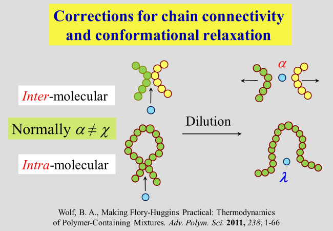
The necessity for such an additional contribution results from the connectivity of polymer segments, in combination with the flexibility of chain molecules. The separation of inter-molecular contacts between segments has already been addressed above. However, intra-molecular contacts will also be opened in good solvents or closed in poor ones to attain the minimum of the Gibbs energy, where the corresponding effect \(\lambda\) differs from alpha.

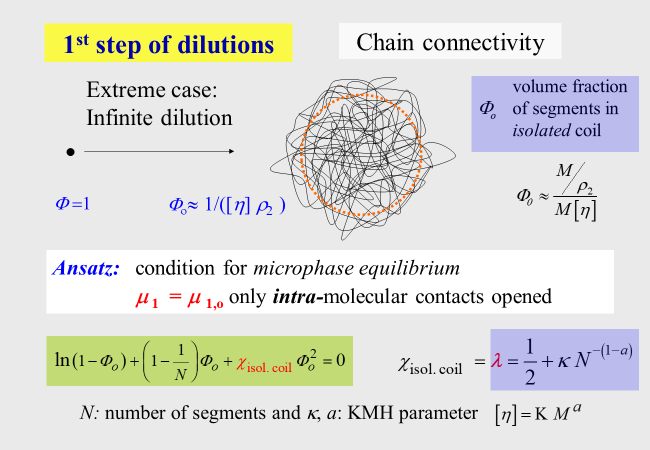
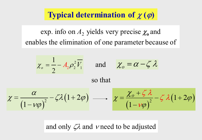
In order to get access to \(\lambda\), we perform an experiment in thought and let a single fully collapsed polymer coil (volume fraction \(\Phi\) of polymer within the realm of this molecule is equal unity) swell in pure solvent up to its equilibrium value \({\Phi _{\rm{o}}}\). Under the reasonable assumption that the specific volume of an isolated coil is in good agreement identical with the hydrodynamic specific volume of the polymer at infinite dilution, it is possible to calculate \({\Phi _{\rm{o}}}\) by means of the intrinsic viscosity of the polymer together with the molar mass M and the density of the pure polymer.

To determine the intra-molecular interaction parameter \(\lambda\), we only need to formulate the equilibrium condition for the solvent (the only component that is able to trespass the hypothetical boundary between the coil-phase and the pure solvent surrounding it). In view of the extremely low polymer concentration within coils we use the original Flory-Huggins theory for that purpose and are now able to calculate \(\lambda\) as a function of the polymer molecular weight by means of the Kuhn-Mark-Houwink relation. At this point it is important to note the principle difference between \(\alpha\) (inter-molecular parameter) and \(\lambda\) (intra-molecular parameter): For good solvents \(\alpha\) < 0.5, whereas \(\lambda\) > 0.5; for poor solvents the opposite is the case.

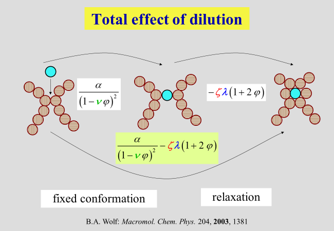
The parameter \(\zeta\) describing the contribution of the second step of dilution, together with the parameter \(\alpha\), quantifies the total effect. For the pseudo-ideal theta conditions, the interaction of all types of segments with the solvent is identical and there is no need for a rearrangement after the first step of dilution; in other words, \({\zeta _\Theta } = 0\). For thermodynamically better than theta-solvents \(\zeta\) is positive for worse it is negative.

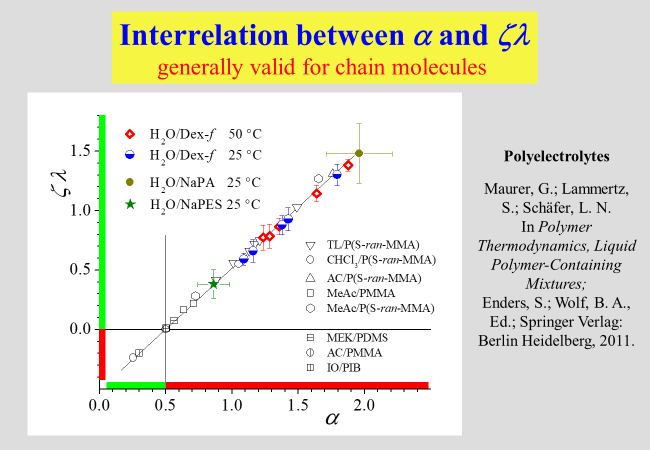
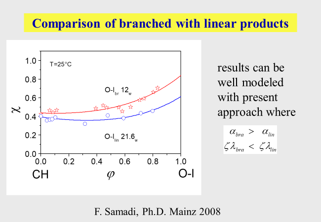
A further helpful finding concerns an interrelation between the parameters \(\alpha\) and the combined parameter \(\zeta \,\lambda\), which obviously holds true for all chain molecules, including polyelectrolytes.

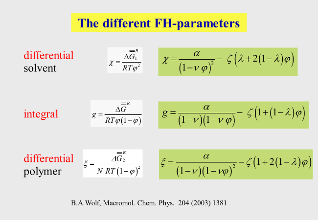
For the useability of this molecular approach it is important to keep in mind that different expressions for the chemical potential of the polymer and for the integral Gibbs energy must be used, if \(\xi\) is a function of \(\varphi\). The relations resulting for the present Ansatz are summarized in the next chart.

The following two examples illustrate how the approach helps the understanding of the thermodynamic behavior of polymers with dissimilar structure and how it can rationalize otherwise inconceivable experimental findings.

The comparison of linear and branched oligo-isoprene[^299] has for instance demonstrated characteristic differences in their interaction with cyclohexane as stated in the following chart.

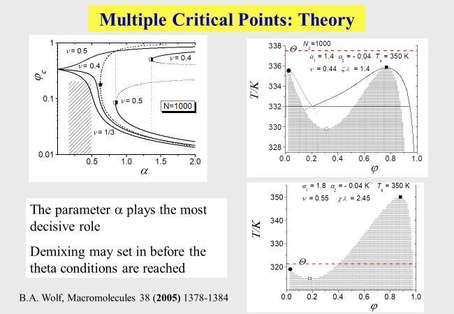
Another advantage of the present approach lies in its ability to explain the reasons for the occurrence of a strange phenomenon, namely the observation of two critical points for binary systems solvent/polymer (Koningsveld, R.; Stockmayer, W. H.; Nies, E. Polymer Phase Diagrams, 1st ed.; Oxford University Press: New York, 2001). These phenomena are caused by a particular combination of the parameters[^263], above all of \(\alpha\) and \(\nu\).

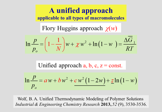
Unified modeling[^318]: All approaches presented so far refer to macromolecules with chain-like structure, where some of them include polyelectrolytes, but none of them can model the solution behavior of globular polymers. In an attempt to find a way to incorporate this type of macromolecules, we have established the following Ansatz: It starts from the Flory−Huggins theory and extends it in a 2-fold manner: The number of segments assigned to the solvent is no longer unity, but is treated as an adjustable parameter to account for the differences in the molecular geometries and in the free volumes of the components. Furthermore, the modeling allows for effects resulting from ternary contacts of the solvent/ polymer/polymer type. The following chart compares the expressions of the original Flory-Huggins theory for the reduced vapor pressures (solvent activity) with that of the unified approach, where the composition variables are weight fractions w instead of the usual volume fractions.

The parameter a can be calculated from the molecular weight of the polymer, b corresponds to \(\chi\) and the parameters c and z are newly introduced. Solutions of proteins and of linear or branched chainlike macromolecules require two adjustable parameters (b and z) for the quantitative thermodynamic modeling; polyelectrolyte solutions also require c.

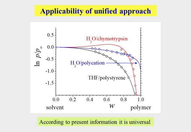
Examination of the thermodynamic expressions displayed above by means of literature data (composition dependent chemical potentials of the solvents) demonstrates their general validity, despite the dramatic differences in the Gibbs energies of mixing for the different types of macromolecules. Also indicated in the graphs are the numbers of segments that need to be assigned to the solvent molecule for a quantitative description of the actual mixing behavior of the system.

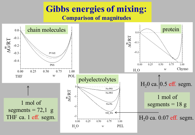
Notwithstanding its simple nature, the unified approach is in a position to describe the measured vapor pressures as a function of composition for all types of polymer/solvent systems tested so far, as demonstrated below for some typical examples.